
The 10 types of Beatles song
With 13 studio albums and a career that spanned more than a decade, The Beatles are not only known for being the best-selling band in history but also for their stylistic range. Although the Fab Four started off as a straightforward - albeit wildly successful - rock and roll outfit, they later broadened their output to include pop ballads, psychedelia and Indian raga rock. Their self-titled LP, released in 1968 and popularly known as ‘The White Album’, represented the height of their eclecticism, as it spanned hard rock (‘Back in the USSR’), ska (‘Ob-La-Di, Ob-La-Da’), country (‘Rocky Racoon’) and experimental (‘Revolution 9’).
 The Beatles in India (Source: Rolling Stone)
For newcomers to the band, such diversity can be overwhelming. It might even appear that The Beatles’ music is uncategorisable – a series of discrete ventures into different genres and subgenres. However, with the power of k-means clustering, we can segment Beatles tracks according to nine acoustic features that are used by Spotify and academic researchers to classify music, namely:
- Acousticness: Probability that a track was produced using acoustic instruments
- Danceability: Based on tempo, rhythm stability, beat strength, etc
- Energy: A measure of frenetic activity
- Instrumentalness: Probability that a track was performed using only instrumental sounds
- Liveness: Probability that a track was performed in front a live audience
- Loudness: Self-explanatory; measured in decibels
- Speechiness: The amount of spoken words in a track
- Tempo: How fast/slow a track is
- Valence: How happy/sad a track is is
Data retrieval and preparation
The first thing we need to do is to retrieve the data. To do this, you need the spotifyr package and a client ID/secret for the Spotify API. To obtain access, follow the instructions on the Spotify for Developers website.
# Load necessary packages
library(spotifyr)
library(tidyverse)

# Load Spotify credentials
Sys.setenv(SPOTIFY_CLIENT_ID = read.csv("~/spotify/spotify_credentials.csv")[1,1])
Sys.setenv(SPOTIFY_CLIENT_SECRET = read.csv("~/spotify/spotify_credentials.csv")[1,2])

# Retrieve access token
access_token <- get_spotify_access_token()
Once we’re hooked into the API, we can use the get_artist_audio_features() function to retrieve The Beatles’ discography. Peeking inside the returned data frame, we can see columns on our audio features of interest – energy, tempo, duration, etc – as well as basic categorical features like album name, album release date and track name.
# Retrieve audio features from Spotify
beatles <- get_artist_audio_features("The Beatles")

# Print the first few rows
head(beatles)
## # A tibble: 6 x 23
## album_uri album_name album_img album_release_d… album_release_y…
## <chr> <chr> <chr> <chr> <date>
## 1 3KzAvEXc… Please Pl… https://… 1963-03-22 1963-03-22
## 2 3KzAvEXc… Please Pl… https://… 1963-03-22 1963-03-22
## 3 3KzAvEXc… Please Pl… https://… 1963-03-22 1963-03-22
## 4 3KzAvEXc… Please Pl… https://… 1963-03-22 1963-03-22
## 5 3KzAvEXc… Please Pl… https://… 1963-03-22 1963-03-22
## 6 3KzAvEXc… Please Pl… https://… 1963-03-22 1963-03-22
## # … with 18 more variables: album_popularity <int>, track_name <chr>,
## # track_uri <chr>, danceability <dbl>, energy <dbl>, key <chr>,
## # loudness <dbl>, mode <chr>, speechiness <dbl>, acousticness <dbl>,
## # instrumentalness <dbl>, liveness <dbl>, valence <dbl>, tempo <dbl>,
## # duration_ms <dbl>, time_signature <dbl>, key_mode <chr>,
## # track_popularity <int>The Beatles’ discography on Spotify includes a lot of live albums and compilation albums that would muddy our analysis. To filter them out, we simply filter for an album_release_date prior to 1971. We can then select our columns of interest and save them in a separate data frame.
# Filter for albums released before 1971
beatles_core <- beatles %>%
  filter(album_release_date < "1971-01-01")

# Filter out bonus tracks on Sgt Pepper's album
beatles_core <- beatles_core[-(111:117),]

# Select track name and acoustic features
beatles_core_metrics <- beatles_core %>%
  select(track_name, danceability, energy, loudness, speechiness,
         acousticness, instrumentalness, liveness, valence, tempo)
Data analysis
Elbow plot
To help us decide how many clusters to choose, we can use the elbow plot technique. Unfortunately, the elbow plot exhibits a smooth curve that does not make it easy to decide how many clusters would be appropriate. Nevertheless, 10 seems an appropriate number, since it sits somewhere in the middle of the elbow region of the plot.
# Set seed for reproducibility
set.seed(1234)

# Scale the data
beatles_core_metrics[2:10] <- scale(beatles_core_metrics[2:10])

# Use map_dbl to run many models with varying value of k (centers)
tot_withinss <- map_dbl(1:30,  function(k){
  model <- kmeans(x = beatles_core_metrics[2:10], centers = k)
  model$tot.withinss
})

# Generate a data frame containing both k and tot_withinss
elbow_df <- data.frame(
  k = 1:30,
  tot_withinss = tot_withinss
)

# Plot the elbow plot
ggplot(elbow_df, aes(x = k, y = tot_withinss)) +
  geom_line() +
  scale_x_continuous(breaks = 1:30) +
  geom_vline(xintercept = 10, linetype = "dashed")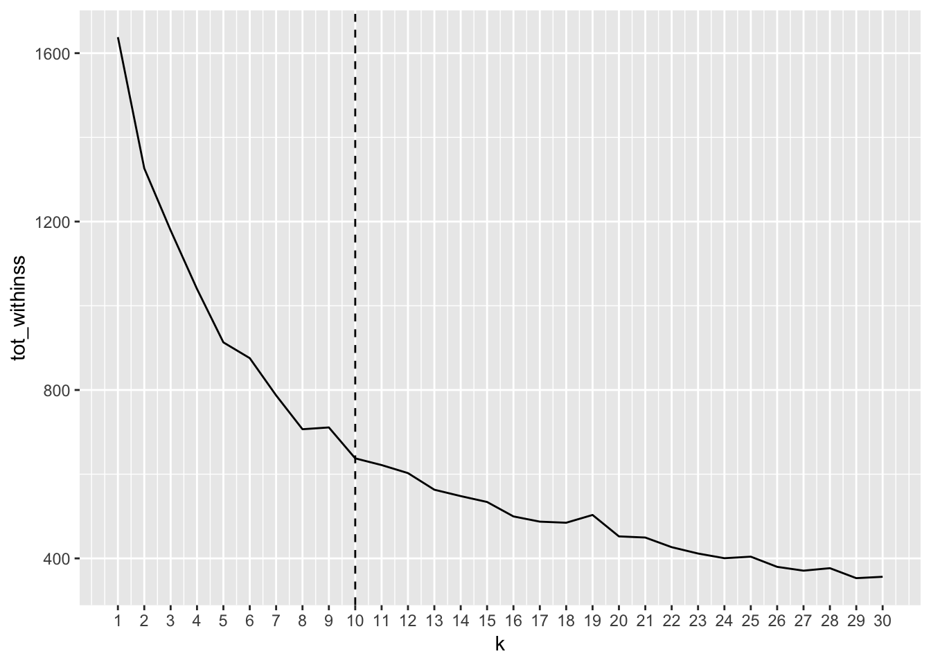
K means
Now that we have decided on how many clusters to use, we can fit our k-means model by using the kmeans function in the built-in stats package.
# Set seed for reproducibility
set.seed(1234)

# Run the model
beatles_k <- kmeans(beatles_core_metrics[2:10], centers = 10, nstart = 100)
We can now assign clusters to each of the tracks and visualise how they differ in key attributes. However, since it is impossible to visualise all of the nine dimensions that we clustered them on, we can only compare two attributes at a time – for example energy and valence.
# Save the clusters
beatles_core_metrics$cluster <- beatles_k$cluster

# Plot energy against valence
beatles_core_metrics %>%
  ggplot(aes(energy, valence, color = as.factor(cluster))) +
  geom_point()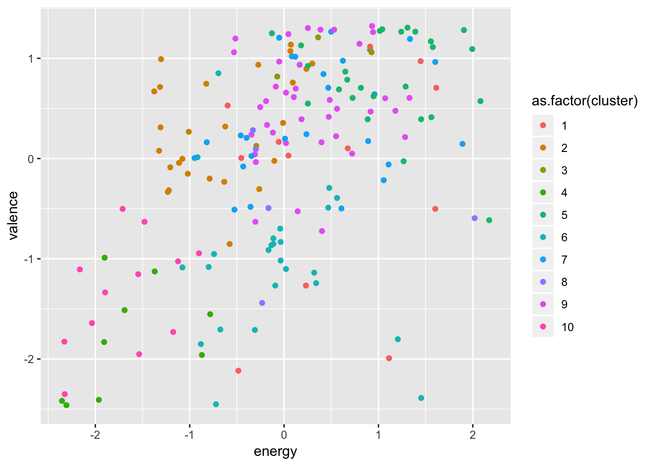
We can get a more detailed impression of the clusters by looking at the matrix of cluster centres. The sign and magnitude of these values give us all the information we need to describe our clusters qualitatively.
# Print cluster centres
round(beatles_k$centers, 2)
## danceability energy loudness speechiness acousticness instrumentalness
## 1 0.07 0.50 0.20 0.55 -0.29 0.00
## 2 1.00 -0.67 -0.33 -0.31 1.10 -0.34
## 3 0.28 0.40 0.31 -0.46 -0.90 3.20
## 4 -0.81 -1.68 -2.39 -0.30 1.22 3.33
## 5 -0.34 1.10 0.66 0.31 -0.20 -0.30
## 6 -0.89 -0.11 0.09 -0.12 -0.75 0.02
## 7 -0.22 0.30 0.45 -0.33 0.05 -0.34
## 8 -0.38 0.20 -0.45 4.75 0.12 0.35
## 9 0.71 0.28 0.39 -0.31 -0.78 -0.32
## 10 -0.80 -1.69 -1.39 -0.29 1.44 -0.30
## liveness valence tempo
## 1 2.84 -0.19 -0.58
## 2 -0.44 0.29 0.04
## 3 -0.09 1.03 -0.05
## 4 0.09 -1.81 -0.88
## 5 0.12 0.82 0.92
## 6 -0.35 -1.04 0.84
## 7 0.23 0.38 -1.06
## 8 0.30 -0.43 0.35
## 9 -0.46 0.54 -0.12
## 10 -0.59 -1.35 -0.22Summary of cluster characteristics
Cluster #1: Performances
 The Beatles performing ‘Get Back’ on the rooftop of Apple Corps at 3 Savile Row (Source: Jeffrey Pepper Rodgers)
- Key features: High liveness
- Number of songs: 12 (7% of total)
- Examples: Get Back; Sgt. Pepper’s Lonely Hearts Club Band; One After 909
With high liveness, Cluster #1 tracks give the impression that they were recorded in front of a live audience. They are energetic and written with the stage in mind.
Cluster #2: Ballads
Songs in Cluster #2 – which I’ve loosely called ‘Ballads’ – come under the broad umbrella of folk rock, often telling wistful tales about colourful characters or romantic interests. The cluster also captures some of The Beatles’ experiments with baroque pop (‘Eleanor Rigby’, ‘For No One’) and music hall (‘When I’m Sixty Four’, ‘Your Mother Should Know’).
- Key features: High acousticness, high danceability
- Number of songs: 27 (15% of total)
- Examples: In My Life; Eleanor Rigby; Michelle
Cluster #3: Interludes
The three tracks in Cluster #3 are statistical anomalies, perhaps too short for their musical features to be reliably expressed. Nothing much to see here.
- Key features: High instrumentalness, high valence, low acousticness
- Number of songs: 3 (2% of total)
- Examples: Birthday; Hey Bulldog; Words Of Love
Cluster #4: Instrumentals
Cluster #4 comprises the instrumental portion of The Beatles’ portfolio. Most of the Yellow Submarine album – the soundtrack to the animated film of the same name – is sorted into this cluster.
- Key features: High instrumentalness, low loudness, low valence
- Number of songs: 9 (5% of total)
- Examples: Pepperland; Sea Of Holes; Sea Of Monsters
Cluster #5: Rockers
Cluster #5 is classic rock and roll, with high energy, high tempo and an upbeat mood. It picks up many of the early Beatles classics (‘Twist And Shout’, ‘I Saw Her Standing There’, ‘Love Me Do’), as well as the band’s later experiments with hard rock (‘Back in the U.S.S.R.’). This is a coherent cluster that works well as a standalone playlist.
- Key features: High energy, high tempo
- Number of songs: 27 (15% of total)
- Examples: Twist And Shout; I Saw Her Standing There; Love Me Do
Cluster #6: Meditations
Several of the tracks in this cluster were penned by George Harrison and show an Eastern or psychedelic influence (‘Tomorrow Never Knows’, ‘Blue Jay Way’). They are often sad and meditative, whether contemplating love and devotion (‘Something’) or the loneliness of a spiritual hermit (‘Dear Prudence’). There is a skew towards The Beatles’ later work, with no tracks from the first four albums.
- Key features: Low valence
- Number of songs: 25 (14% of total)
- Examples: Here Comes The Sun; Something; Dear Prudence
Cluster #7: Slowcoaches
Cluster #7 is distinguished by its slow tempo, with languorous songs including ‘Dig A Pony’ (59 bpm), ‘Little Child’ (76 bpm) and ‘All My Loving’ (78 bpm). A fifth of the tracks are from the band’s second album, ‘With the Beatles’.
- Key features: Low tempo
- Number of songs: 25 (14% of total)
- Examples: All You Need Is Love; Yellow Submarine; Hello, Goodbye
Cluster #8: Vignettes
This small cluster picks up some of The Beatles’ more lyrically dense tracks, primarily characterised by their descriptiveness and emphasis on the spoken word.
- Key features: High speechiness
- Number of songs: 25 (3% of total)
- Examples: Strawberry Fields Forever; Polythene Pam; Maggie Mae
Cluster #9: Middlers
Cluster #9 sits somewhere between the hard rock sound of Cluster #5 and the folk rock sound of Cluster #2. It has no distinguishing features, with fairly average loadings for all nine of the acoustic features. It is the most populous cluster, representing 21% of The Beatles’ discography.
- Key features: None
- Number of songs: 38 (21% of total)
- Examples: Help!; A Hard Day’s Night; Eight Days A Week
Cluster #10: Lullabies
Cluster #10 is a collection of sleepy gems from The Beatles’ catalogue and works well as a standalone playlist (aside from the intrusion of ‘Her Majesty’ towards the end). Primarily characterised by a low energy, it is a nice assortment of songs to drift away to.
- Key features: Low energy, high acousticness, low loudness
- Number of songs: 12 (7% of total)
- Examples: Yesterday; Blackbird; Golden Slumbers
Concluding remarks
K-means clustering has done a decent job of organising The Beatles’ diverse discography into a set of coherent segments. The nine audio features describe the tracks with some accuracy, allowing the algorithm to make sensible groupings.
That said, the method does occasionally cluster on features that – although descriptive in a technical sense – do not convey the true mood or timbre of the music. For example, Cluster #8 is distinguished by ‘speechiness’, but the songs it captures would likely be placed elsewhere if sorted by hand. This is a problem with the the data itself rather than the algorithm.
A more comprehensive clustering could take into account the lyrics of each song, which we can imagine would help to group together songs about, for example, love and relationships. Even so, the current method has proved an effective means of studying one of the most eclectic rock portfolios in music history.


